Finding the brachistochrone with JAX

Here’s the brachistochrone problem:

What path yields the shortest duration for a ball to roll from A to B?

The shortest path from A to B is a straight line, but it’s actually not the fastest path:

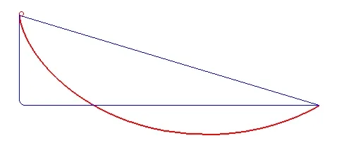
We can get better results by accelerating the ball down a steeper path at first, then taking a bit of a loss as the ball rolls down the more shallow latter part of the path. The optimal solution to this problem is a cycloid. Can we arrive at the optimal path numerically instead? What if we use gradient descent?

JAX is a library that provides a numpy-like API, but automatically differentiable and following the functional programming paradigm. JAX lets us easily compute the gradient of a function written in numpy-like syntax, for example:

def f(x):
	return jnp.sum(x**2)

x = jnp.array([0., 1., 2.])
grad_f = jax.grad(f)
print(grad_f(x)) # [0., 2., 4.]

Being able to evaluate the gradient with just a single grad function call means we can just as easily evaluate the gradient of a function that computes the time for a ball to roll down a curve. The inputs to our function can be the curve itself, which we’ll represent as an array of y-values corresponding to equally-spaced x-values. In other words, the value of the i-th element in the array ys is the height of our experimental curve at x=i.

# Computes the time to each segment at heights specified by `ys`
def t(xs, ys):
  vs = jnp.sqrt(2 * G * (Y_0 - ys)) # velocity
  midpt_v = (vs[1:] + vs[:-1]) / 2. # velocity at the midpoint of each arc length
  dys = ys[1:] - ys[:-1] # difference between heights for each segment
  dx = xs[1] - xs[0]
  arc_lengths = jnp.sqrt(jnp.power(dx, 2) + jnp.power(dys, 2)) # euclidean distance as arc length
  return jnp.cumsum(arc_lengths / midpt_v) # sum times as t approaches infinity

If we repeatedly nudge the curve in the direction of this gradient, we should converge on an optimal solution to the brachistochrone problem. We already wrote an automatically differentiable (thanks to JAX) function to evaluate the time t it takes for the ball to roll from the start to the end of our curve. Now let’s find out how to nudge each element in ys in order to minimize t:

def loss(params):
  ts = t(xs, params)
  t_final = ts[-1]
  return t_final

loss_grad = jax.grad(loss)

def optimize(params, LR=0.01, N_STEPS=1000):
  for _ in range(N_STEPS):
    grads = loss_grad(params)
    params = jnp.concatenate([
      jnp.array([Y_0]),
      params[1:-1] - (LR * grads[1:-1]),
      jnp.array([0])
    ])

N_STEPS = 3000
LR = 0.02
optimize(ys, LR=LR, N_STEPS=N_STEPS)

Our solution should roughly converge on the optimal path: